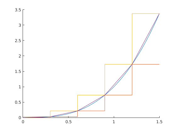
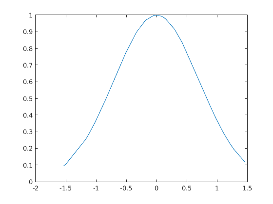
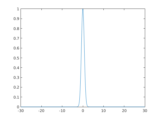
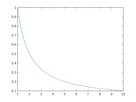
%MATLAB ASSIGNMENT 1 : INTEGRALS

%-------------PART 1: Riemann sums with fixed lengths---------------
disp('-----------------Part 1-------------------------');
f = @(x) x.^3;  %this defines a function f of a single variable x

%What is the exact value of the integral of f from 0 to 1.5?
%Compute it by hand, and store the result in a variable.

exactValue = 1.5^4/4			%<--- your answer here

figure('Name','Riemann sums'); %this line creates a new figure
hold on;%tells Matlab to display several plots on the same figure

%Plot f on the interval [0..1.5]

t=[0:0.01:1.5];
plot(t,f(t));

%Compute the left Riemann sum for f on the interval [0..1.5] with N=5
%(i.e. by subdividing it into N = 5 intervals of equal length).

N = 5;
%Compute dx, the length of the sub-interval (aka steps size), in terms of N
dx = (1.5 - 0)/N;
%Set up an array with x values ranging from 0 to 1.5 with step size dx
x=[0:dx:1.5];
%Store the first N values (all but last) in another array
xLeft = x(1:end-1);
%Compute the sum using the array with the first N values
sumLeft = sum(f(xLeft).*dx)


%Is this an overestimate or underestimate? Why?
disp('This is an UNDERestimate because the function is increasing on 0..1.5');
%The following function will plot a staircase graph (don't worry about how it works):
steps = @(x,y) plot(reshape([x(1:end-1);x(2:end)],1,[]),reshape([y;y;],1,[]));

%Usage: steps(x,y)
%x - an array of numbers
%y - an array of numbers, having one less value than x

%output: plots the step function whose value on [x(i)..x(i+1)] is y(i)
%        for i=1..length(x)
%Example (run this script, then type in command line):
%steps([1 2 3 4], [1 2 3])

%The left Riemann sum can be seen as the area under a staircase plot
%Use the steps function above to plot this staricase.
%Hint: use the array with all x values as the first argument,
%and array with values of f on the left endpoints as the second argument.
steps(x,f(xLeft));

%Compute the right Riemann sum for f on the inteval [0..1.5] with N = 5
xRight = x(2:end);
sumRight = sum(f(xRight).*dx)
%Plot the step-function whose area is given by this sum
steps(x,f(xRight));
%Is this an overesimate or underesimate? Why?
disp('This is an OVERestimate because the function is increasing on 0..1.5');

%Compute the averate of the above two sums.
%This is called the "trapezoid approximation", since the mean of areas of
%two rectangles with the same base is the area of the trapezoid.
sumTrap = (sumRight + sumLeft)/2
%Is this an overestimate or underestimate? Why?
disp('This is an OVERestimate because the function is CONCAVE UP on 0..1.5');

%This approximation is simply the area of the piecewise-linear
%approximation obtained by connecting the dots (x0,f(x0)), (x1,f(x1)),..

%Plot this piecewise linear function. Hint: plot(x,y)
%does what you want: connects (x(1), y(1)), (x(2),y(2)), (x(3),y(3)),...
plot(x,f(x));

%What is the error, as a percentage of the true value?
%That is, if ST is the trapezoid sum, and A is the value of the integral,
%find |ST-A|/A
error = abs((sumTrap - exactValue)/exactValue)

%Experiment by changing the value of N above. Set N = 10,20,30 and re-run the script.
%What happens to approximation as N increases?
disp('Approximation becomes more precise as N increases.');

%Which value of N gives approximation that within 0.0001 of the true
%value?

disp('N=10000 is good enough for an answer within 0.0001 of the true value.');

%-----------PART 2: integrals from data--------------------------------------
figure('Name', 'Integrals from data');

%You are given the following numberic data (gx contains the values of g(x) for some function g)
x=[-1.53791054834832,-1.49569810068615,-1.16989017405482,-1.14255885947370,-1.13895608794648,-1.12132996518602,-1.01239961679621,-0.845644131020566,-0.751398018530839,-0.511654284156889,-0.507415971326562,-0.344861415487210,-0.316428672889217,-0.185957360453133,-0.173007337607668,-0.0460550662940558,0.00635141688703844,0.0837915499445878,0.104852877827265,0.148214568125196,0.298266503318215,0.425661058965354,0.798414645773748,0.875818517048553,0.948581873231802,0.985349484833958,1.11465121173926,1.21024273817800,1.27955837883071,1.46202681067196];
gx=[0.0939334379248379,0.106766314619003,0.254452011841628,0.271053042801056,0.273290220347042,0.284397921108716,0.358813334945164,0.489136348869598,0.568588114970200,0.769672556024332,0.773004067874842,0.887870485852825,0.904722415960850,0.966010920559311,0.970511973624385,0.997881178746198,0.999959660317194,0.993003565963587,0.989066088543726,0.978271971435618,0.914879508569152,0.834279052620699,0.528630305626131,0.464377223760203,0.406647903377131,0.378736863244691,0.288676866957447,0.231150218028945,0.194510400404625,0.117946706646648];

%Plot gx vs x
plot(x,gx);
%the values of x are in range [-pi/2..pi/2], and y=g(x) for some
%funciton g. Approximate integral of g from -pi/2 to pi/2 by computing
%the left and right riemann sums and their average.
%You already have f evaluated on the subdivision, the only thing
%different from before is that the intervals in the subdivision have
%varying lengths. The diff() function can be used to compute them.
disp('-----------------Part 2-------------------------');
%Left Riemann sum:
sumLeft = sum(gx(1:end-1).*diff(x))
%Right Riemann sum:
sumRight = sum(gx(2:end).*diff(x))
%Average of these sums:
sumT = (sumLeft + sumRight)/2
%Plot the step function

%-----------PART 3: random sampling--------------------------------------
figure('Name','Random sampling')
h = @(x) exp(-x.^2); %this is an example of a Gaussian function. This might
                     %be familiar to you as the "Bell Curve"


N = 10000;

a = -30;
b = 30;
xn = sort(rand(N,1)*(b-a)) + a; %this generates an array of N random numbers in the interval [a..b]
                                %sorted in increasing order

%plot h on [a..b]
t = [a:0.001:b];
plot(t,h(t));

%Compute the left Riemann sum, right Riemann sum and their average.
%Since the differences between successive points are not the same, use
%the diff() funciton to obtain a list of differences.
disp('-----------------Part 3-------------------------');
%Left Riemann sum:
sumLeft = sum(h(xn(1:end-1)).*diff(xn))
%Right Riemann sum:
sumRight = sum(h(xn(2:end)).*diff(xn))
%Average of the two (a.k.a. trapezoidal approximation):
sumT = (sumLeft + sumRight)/2
%Compute the square of this approximation:
approxSqr = sumT.^2

%Increase N to 500, 1000, 10000. Does the square of the approximation seem
%to approach anything?
disp('The approximation approaches pi.');

%-------------------------PART 4: Exploring--------------------
figure('Name', 'Exploring 1/x');
f = @(x) 1./x; %we'll study the integral of this function by crunching numbers

%plot f from 1 to 10
t = [1:0.001:10];
plot(t,f(t));

a = 1.5;
b = 2.5;
%approximate the integral of f by a left Riemann sum with dx=0.001
%on intervals [1..a], [1..b], [1..a*b]

dx=0.001;

%Array with x values from 1 to a with step dx:
xa = [1:dx:a];

%Array with x values from 1 to ab with step dx
xb = [1:dx:b];

%Array with x values from 1 to a*b with step dx
xab = [1:dx:a*b];

%Area under the curve from 1 to a (approximate by a Riemann sum with step dx):
Sa = sum(f(xa).*dx)

%Area under the curve from 1 to b (approximate by a Riemann sum with step dx):
Sb = sum(f(xb).*dx)

%Area under the curve from 1 to a*b (approximate by a Riemann sum with step dx):
Sab = sum(f(xab).*dx)

%Try several more values of a and b (change them above),
%and record results in the table below:

disp('  Sa   |   Sb  |   Sab');
disp('-------|-------|--------');
disp('1.5047 | 1.2534|2.7574');
disp('0.6939 | 0.6939|1.3869');
disp('2.4854 | 1.6100|4.0949');

%What conclusion can you make about relationship between Sa, Sb and Sab ?

disp('Sab = Sa * Sb');

%Let An be the area under the curve on the interval [1..2^n]
%Compute An for n = 1 2 3 4 via a Riemann sum approximation with step dx

x = [1:dx:2];
A1 = sum(f(x).*dx)
x = [1:dx:4];
A2 = sum(f(x).*dx)
x = [1:dx:8];
A3 = sum(f(x).*dx)
x = [1:dx:16];
A4 = sum(f(x).*dx)

%Plot n vs. An for n = 1, 2, 3, 4
n = [ 1 2 3 4];

An = [A1 A2 A3 A4];
figure('Name', 'Plot of A_n for n=1..4');
plot(n, An);
%What conclusion can you make from this about the value of An?

disp('Conclusion: A_n = n*A_1.');

%Recall that if 2^y = x, then y = log_2(x)
%Therefore, integral_1^x f(t) dt = A_?    (fill in the question mark)
disp('=> integral_1^x f(t) dt = A_{log_2(x)}');
%Using this and your observation above, write a formula for
% integral_1^x f(t) dt  in terms of A_1.
disp('So integral_1^x f(t) dt = log_2(x) * A_1.');
-----------------Part 1-------------------------
exactValue =
1.2656
sumLeft =
0.8100
This is an UNDERestimate because the function is increasing on 0..1.5
sumRight =
1.8225
This is an OVERestimate because the function is increasing on 0..1.5
sumTrap =
1.3162
This is an OVERestimate because the function is CONCAVE UP on 0..1.5
error =
0.0400
Approximation becomes more precise as N increases.
N=10000 is good enough for an answer within 0.0001 of the true value.
-----------------Part 2-------------------------
sumLeft =
1.7182
sumRight =
1.7052
sumT =
1.7117
-----------------Part 3-------------------------
sumLeft =
1.7712
sumRight =
1.7737
sumT =
1.7724
approxSqr =
3.1416
The approximation approaches pi.
Sa =
0.4063
Sb =
0.9170
Sab =
1.3224
Sa | Sb | Sab
-------|-------|--------
1.5047 | 1.2534|2.7574
0.6939 | 0.6939|1.3869
2.4854 | 1.6100|4.0949
Sab = Sa * Sb
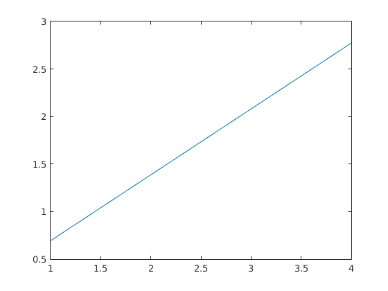
A1 =
0.6939
A2 =
1.3869
A3 =
2.0800
A4 =
2.7731
Conclusion: A_n = n*A_1.
=> integral_1^x f(t) dt = A_{log_2(x)}
So integral_1^x f(t) dt = log_2(x) * A_1.