%%MATLAB ASSIGNMENT 2: DERIVATIVES REVISITED

%Welcome to MATLAB assignment 2, where calculus is made real

%The "real" numbers as you know them are an illusion, or a very useful
%convention. The physical universe doesn't allow for arbitrary small
%values. So, for this assignment, we just agree that the smallest value
%we'll deal with is...

dx = 0.0001;

%..and use it to define everything else. For example, the differential:

d = @(f,x) f(x+dx) - f(x);

%d(f,x) computes df(x). You have seen the notation "du" in your
%substituiton rule, but it was very loosely defined. Here, df(x) is a very
%concrete difference.

%What is this difference good for? Well, the derivative is just the ratio
%df/dx. See for yourself:

f = @(x) x.^2; %we define a function f = x^2
should_be_six = d(f,3)/dx %this computes df/dx(3) -- what should the value be?

%This lab will revisit the derivative and its connection to the integral.
should_be_six =

    6.0001
%PART 1: THE FUNDAMENTAL THEOREM OF CALCULUS
%-------------------------------------------------------------------------
%Define a function int(f,a,b) that computes the integral numerically with
%step size equal to dx
%int(f,a,b) should return the integral of f from a to b
%HINT: use your knowledge from previous lab. You don't need to bother with
%left / right sums since the value of dx is small; an extra summand won't
%affect the precision much.

%You can put an anonymous function definition here, or make a function file.

%If you choose to do it with an anonymous function,
int = @(f,a,b) sum(f([a:dx:b])).*dx;
%Define a function f  = x^3. Compute its integral from 0 to 1 using your
%function. Verify that the value is what it should be.
f = @(x) x.^3;
%Integral of f from 0 to 1 using your int():
int_f_0_1 = int(f,0,1)
%True value (computed by hand):
true_value = 1/4
%Here, I define a new function in terms of yours:

df = @(x) d(f,x);
int_f_0_1 =

    0.2501


true_value =

    0.2500
%Compute the integral of df(x)/dx from 0 to 1, 2, 3 using your integral
%function. Verify that the values are what they should be according to FTC.
%   HINT: define a new function g = df(x)/dx, and integrate it.
%Alternatively, compute the integral of df, and divide by dx
%(MATLAB is stupid, and df./dx is not a valid expression in MATLAB)

g = @(x) df(x)./dx;
%Integral of df from 0 to 1:
int_df_1 = int(g,0,1)
int_df_1 =

    1.0003
%Should be equal to this according to FTC:
v1 = f(1) - f(0)
v1 =

     1
%Integral of df from 0 to 2:
int_df_2 = int(g,0,2)
int_df_2 =

    8.0012
%Should be equal to this according to FTC:
v2 = f(2) - f(0)
v2 =

     8
%Integral of df from 0 to 3:
int_df_3 = int(g,0,3)
int_df_3 =

   27.0027
%Should be equal to this according to FTC:
v3 = f(3) - f(0)
v3 =

    27
%Let's go the other way around!
%Define F = integral from 0 to x of f using your int function
%(F is a function of x)
F = @(x) int(f,0,x);
%Now compute d/dx(F(x)) for x = 1, 2, 3 USING the d(f,x) function defined
%above, Verify that the values are what they should be.
%   NOTE: use the d() function to compute this numerically
%d/dx(F(x)) at x = 1 is...
f1=d(F,1)./dx
f1 =

    1.0003
%Should be equal to this according to FTC:
v1 = f(1)
v1 =

     1
%d/dx(F(x)) at x = 2 is...
f2=d(F,2)./dx
f2 =

    8.0012
%Should be equal to this according to FTC:
v1 = f(2)
v1 =

     8
%d/dx(F(x)) at x = 3 is...
f3=d(F,3)./dx
f3 =

   27.0027
%Should be equal to this according to FTC:
v1 = f(3)
v1 =

    27
%PART 2: THE SUBSTITUTION RULE
%-------------------------------------------------------------------------

%define a function u = x^2

u=@(x)x.^2;
%Compute the integral of cos(u(x)) du from 0 to sqrt(pi/6) using your the
%d() function defined above and your int() function
%   HINT: define a function g  = cos(u(x)) du(x)/dx, (use the d() function!),
%   and plug it into your int().
%   This will compute integral of cos(u(x)) du/dx dx = cos(u) du
%   NOTE: don't differentiate / integrate by hand.

g = @(x) cos(u(x)).*d(u,x)./dx;

int_f = int(g,0,sqrt(pi/6))
int_f =

    0.5001
%Verify that the integral is what it should be according to the substitution rule.
%What should the value of the integral be? (now, compute it by hand):
true_value = 0.5
true_value =

    0.5000
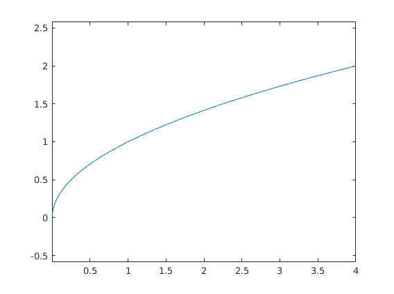
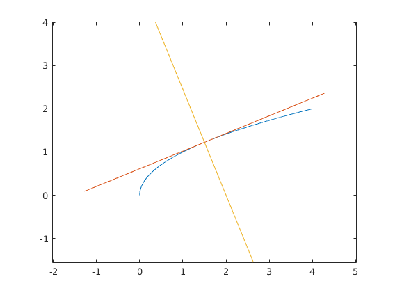
%PART 3: WE DIDN'T LIE, DERIVATIVES REALLY GIVE YOU TANGENTS
%-------------------------------------------------------------------------
figure('Name', 'Tangent and normal');

%Define  f = sqrt(x) and plot it between 0 and 4

f= @(x) sqrt(x);
t=[0:0.001:4];
plot(t,f(t));

hold on;
axis equal;      %sets axis scaling to 1:1 (so the figure is not stretched)
%Use the segment command to draw the TANGENT line to the plot at x = 1.5
%   HINT: the slope is df/dx, so the direction vector is (dx, df)
x = 1.5;
segment(x,f(x),dx,d(f,x),3);
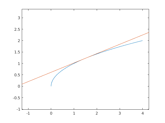
%Use the segment command to draw the NORMAL line to the plot at x = 1.5
%   HINT: the slope is -dx/df
segment(x,f(x),-d(f,x),dx,3);
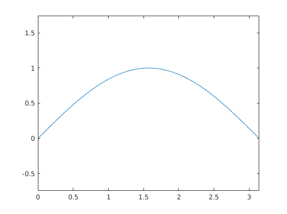
%PART 4: ...AND TANGENTS GIVE YOU DERIVATIVES
%-------------------------------------------------------------------------
%Here we illustrate that the slope of the secant lines approaches the
%derivative.
%
%Set f(x) = sin(x) and plot it between 0 and pi
figure('Name', 'Derivative as limit of tangents');
f  = @(x) sin(x);
t = [0:0.001:pi];
plot(t,f(t));

hold on;
axis equal;
%Now, we'll plot N secant lines with a FOR loop
N = 20;

%The secant lines go through (x0, f(x0)) and (x1, f(x1))
%x0 will be fixed:
x0 = pi/3;
%x1 will take different values between MAX=2 and x0 in the loop
MAX = 2;
for i = 0:N-1 %i runs from 0 to N-1
    x1 =  MAX - (MAX-x0)*i/N;
    %Compute the direction vector:
    %DX is the difference in X values:
    DX = x1 - x0;
    %DY is the difference in Y values:
    DY = f(x1) - f(x0);
    %Use the segment command to plot the tangent line:
    segment(x0,f(x0),DX,DY,2);
end
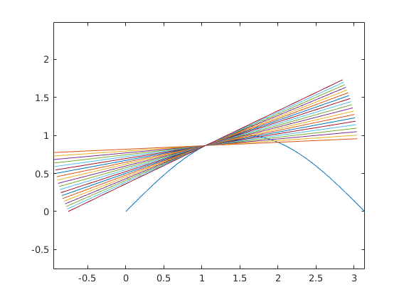
%Output DY/DX (this is last value it has taken in the loop)
%and compare it to df/dx at x0
last_secant_slope = DY/DX
tangent_slope = d(f,x0)./dx
last_secant_slope =

    0.4792


tangent_slope =

    0.5000
%PART 5: ENVELOPE
%-------------------------------------------------------------------------
figure('Name', 'Envelope');

%define f = x^2 and plot it between -1 and 1
f = @(x) x.^2;
x=[-1:dx:1];
plot(x,f(x))

hold on ;
axis equal;
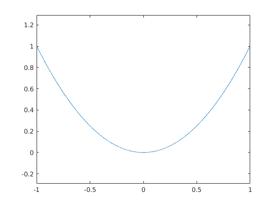
%Draw tangents at 100 points between -1 and 1
%   HINT: set up an array, and use a for loop to loop through it
%   NOTE: pick a nice value for L in the segment command - somethine
%   between 2 and 5, for example - whatever you think looks good
for t=[-1:0.02:1]
   segment(t,f(t),dx,d(f,t),5);
end

%We say that the parabola is an envelope of its tangent lines.
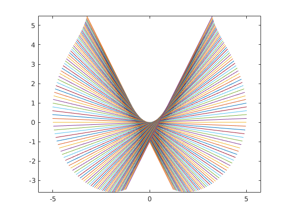
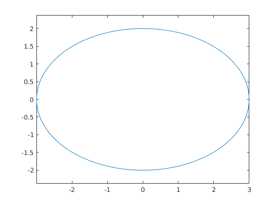
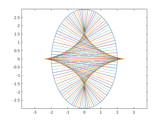
%PART 6: PARAMETRIC CURVE AS AN ENVELOPE OF ITS TANGENTS
%-------------------------------------------------------------------------
dt = dx;
t = [0:dt:2*pi];

figure('Name', 'Parametric envelope');
%The following defines and plots an ellipse
x1 = @(t) 3*cos(t);
x2 = @(t) 2*sin(t);
plot(x1(t),x2(t));
axis equal;
hold on;
%Draw tangents at 100 equally spaced values of t between 0 and 2*pi
%   HINT: set up an array, and use a for loop to loop through it
for t=linspace(0,2*pi,100)
   DX = d(x1,t);
   DY = d(x2,t);
   segment(x1(t),x2(t),DX, DY,5);
end
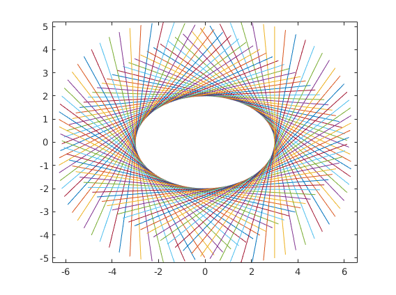
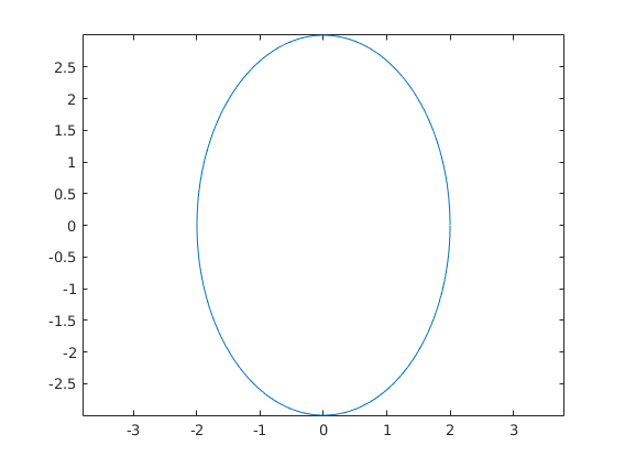
%PART 6: PARAMETRIC CURVE NORMALS
%-------------------------------------------------------------------------
figure('Name', 'Normals to a curve');
%The following defines and plots an ellipse
x1 = @(t) 2*cos(t);
x2 = @(t) 3*sin(t);
t=[0:0.01:2*pi];
plot(x1(t),x2(t));

axis equal;
hold on;
%Draw normals at 100 equally spaced values of t between 0 and 2*pi
%   HINT: set up an array, and use a for loop to loop through it
%   NOTE: set the L argument of the segment command to be 5 or greater for
%   a nice picture
for t=linspace(0,2*pi,100)
   DX = d(x1,t);
   DY = d(x2,t);
   segment(x1(t),x2(t),-DY, DX,5);
end
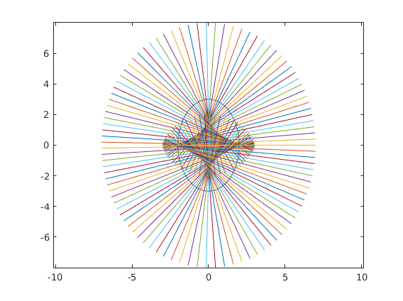
%Notice the shape that is formed inside. Is it smooth? Describe it here:
%Extra credit: define 5 closed parametric curves. Try making a conclusion
%about the shape in the middle: what is a characteristic shared by all
%of them?


%%PART 7: EVOLUTES ------> EXTRA CREDIT, WORTH 1/2 LAB
%This section is a study of the curve in the previous section.
%If you think about it, what your eyes see is the curve formed by
%intersection points of consecutive normals. That is, the evolute is the
%<b>envelope</b> of the normals. Now, we just have to do the opposite of
%what we did in parts 4 and 5: given a family of lines, we construct
%a curve to which they are all tangent.
%The tedious part: given two lines:
%L0 goes through (x0, y0) and has direction vector (a0, b0)
%L1 goes through (x1, y1) and has direction vector (a1, b1)
%What are the coordinates of the intersection point P?
%P satisfies: P = [x0 y0] + t0[a0 b0] = [x1 y1] + t1[a1 b1]
%for some constants t0, t1. Set up and solve the system of linear equations
%for t0 and t1; obtain P as a function of all other variables

P = @(x0,y0,a0,b0,x1,y1,a1,b1) [x0; y0] + [a0 0; b0 0]*([a0 -a1; b0 -b1]\[x1-x0; y1-y0]) ;
%Use the function P to define a function PN which, given functions
%x(t) and y(t) and values t0, t1, computes the intersection of normals
%at t = t0 and t = t1

PN = @(x,y,t0,t1) P(x(t0),y(t0),-d(y,t0),d(x,t0),x(t1),y(t1),-d(y,t1),d(x,t1));
%Now we can use the function P to compute the points we want to plot.
%(That's  the fun part! :) )
%First, we define a curve:
figure('Name', 'Evolute of an ellipse');
x = @(t) 2*cos(t);
y = @(t) 3*sin(t);
N=100;

%Define an array t of size N with numbers going from 0 to 2*pi
t = linspace(0,2*pi,N);

%Plot (x(t), y(t))
plot(x(t),y(t));
axis equal;
hold on;

ex=zeros(N-1,1); %allocate an array for evolute x-points
ey=zeros(N-1,1); %allocate an array for evolute x-points
 for i=1:N-1
        %compute the intersection of normal through t(i) and t(i+1)
        intersection = PN(x,y,t(i),t(i+1));
        %store the intersection point
        ex(i) = intersection(1);
        ey(i) = intersection(2);
        %connect the intersection point to the point on the curve at t(i)
        %HINT: plot([a c], [b d]) connects (a, b) to (c, d)
        plot([x(t(i)) ex(i)], [y(t(i)) ey(i)]);
 end
%plot the evolute
plot(ex, ey);
%Extra Extra credit (worth 1/4 of the lab), plus you get to make something
%Wikipedia-article worthy
%
%Some math background first.
%
%The method of construction of the evolute above reveals its interesting
%property: it is the locus of the centers of the osculating circles,
%the circles that "kiss" the curve (from Latin "osculare" - to kiss).
%
%OK, hold on, let's talk about what this means first.
%
%
%Just like there are tangent lines, there are tangent circles.
%Unlike a tangent line, a circle tangent to a point is not unque - you can
%draw many, by changing the radius (line can be thought of as a tangent
%circle with infinite radius).
%
%If you draw a lot of circles and zoom at the common tangent point, you
%will see that the larger circles are going on the _outside_ of the curve,
%and the smaller circles are on the _inside_.
%The one circle that is in between in the osculating circle.
%It it the limit of the circles going through three points on the curve
%as they approach each other.
%
%Note for physics people: a car going around the curve with unit speed will
%experience the same acceleration at a point (x, y) as the car going around
%the osculating circle at that point with the same speed.
%
%We say that the curve at that point and the circle have the same _curvature_.
%
%In other words, just as the line is the best linear approximation, the
%circle is the best quadratic approximation.
%---------------------------------------------------------------------------

%Write a circ(cx, cy, r) function that plots a circle of radius r centered at (cx, cy)
%HINT: see how the ellipse is plotted.

circ = @(cx, cy, r, w) plot(cx + cos([0:0.1:2.1*pi])*r, cy+sin([0:0.1:2.1*pi])*r);

%Write a function dist(x0, y0, x1, y1) that computes the distance
%from (x0, y0) to (x1, y1)
dist = @(x0,y0,x1,y1) sqrt((x1-x0).^2 + (y1-y0).^2);


%Time to get things moving!
figure('Name', 'Evolute animated!');
for i = 1:N-1 %this sets up the animation loop. Each iteration will draw a new frame.
   %Plot the original curve (x(t), y(t)):
   plot(x(t),y(t));
   axis equal;
   axis ([-8 8 -6 6]);
   hold on;
   %Plot a part of the evolute from time t=t(1) to t = t(i)
   %[NOTE: use the ex, ey arrays that are already computed
   plot(ex(1:i),ey(1:i));
   %Compute the radius of curvature R at time t=i
   %(this is the distance from the point on the curve at time t=t(i) to the corresponding
   % point on the evolute):
   R = dist(ex(i),ey(i),x(t(i)),y(t(i)));
   %Draw a circle of radius R centered at the point on the evolute at time t(i):
   circ(ex(i),ey(i),R,1);
   %Plot a segment connecting the center of the circle to the correspoing
   %point on the curve (to which it will be tangent):
   plot([x(t(i)) ex(i)], [y(t(i)) ey(i)]);


   hold off; %allow the next frame to overwrite the figure
   pause(1/24); %pause before the next frame gets drawn

   %The code below saves the animation to an animated gif file.
   %Once you get the animation right, uncomment these lines
   %to get a nice .gif file that you can post on your Tumblr.
   %Submit the GIF file along with the assignment (ideally, edit the
   %published HTML file to include instead of the static figure).
   %------------------------------------------------------------------
   %[A,map] = rgb2ind(frame2im(getframe(1)),256);
   %if i == 1;
   %imwrite(A,map,'evolute.gif','gif','LoopCount',Inf,'DelayTime',1/24);
   %else
   %	imwrite(A,map,'evolute.gif','gif','WriteMode','append','DelayTime',1/24);
   %end
end