Contents

Assignment 5

%Welcome to assignment 5! This assignment is all about Taylor polynomials.
import tests.* %this allows us to call the test functions from another file

Testing factorials

fact_test_1();
fact_test_2();

Testing fact():
0! = 1, 5! = 120, 7! = 5040
Testing fact() : computing binomial coefficients
The fifth row of Pascal triangle is:
     1     5    10    10     5     1

Testing polynomial evaluation

eval_test_1();
eval_test_2();

Testing eval() with p(x)=2 + 3x + 5x^2 + 7x^3:
p(0) = 2, p(1) = 17, p(2) = 84 
Testing eval() with p(x)=1 + x + x^2 + ... + x^n:
p(1/2) = 1.998047e+00 (should be approximately ___)
p(1/3) = 1.499975e+00 (should be approximately ___)
p(1/5) = 1.250000e+00 (should be approximately ___)

Testing vectorized polynmomial evaluation

vect_eval_test_1();
vect_eval_test_2();

Testing vect_eval() with p(x)=2 + 3x + 5x^2 + 7x^3:
p(x) for x = [0 1 2] is:
     2    17    84

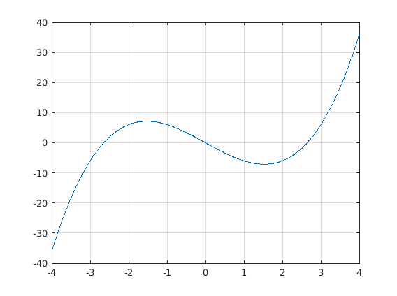
Testing vect_eval() with p(x)=x^3 - 7x to plot p(x):

Testing taylor polynomial

taylor_test_1();
taylor_test_2();
taylor_test_3();
taylor_test_4();

Testing taylor_poly(), test1:
    @(x)2+3*x.^2+5*x.^3+7*x.^4

T4 of f should be [2 0 3 5 7]:
    2.0000    0.0030    3.0150    5.0420    7.0000

Testing taylor_poly(), test 2:
T5 of sin(x) should be ____
         0    1.0000   -0.0005   -0.1667    0.0001    0.0083

Testing taylor_poly, test 3:
T5 of log(x) around x=1: 
         0    0.9995   -0.4990    0.3318   -0.2480    0.1828

Testing taylor_poly, test 4:
T5 of sqrt(x) around x=1: 
   1.0e+11 *

         0    0.0000   -0.0000    0.0000   -0.0058    1.0921

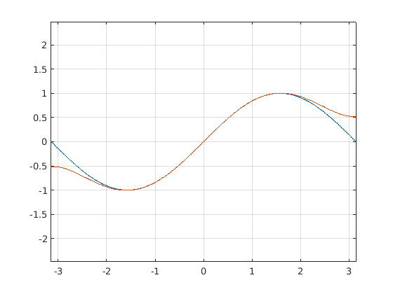
Testing plotting taylor polynomial, part 1

plot_compare_test_1();

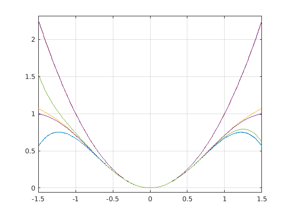
Testing plotting taylor polynomial, part 2

plot_compare_test_2();

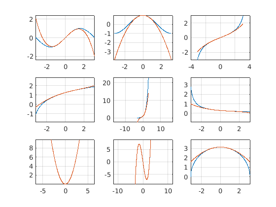
Taylor plot bonanza!

%Compares plots various functions with plots of T3 for them
taylor_plot_bonanza();

Functions

function [nf] = fact(n)
%FACT computes a factorial of a number
%INPUT: n : natural number
%OUTPUT: n! = n(n-1)(n-2)...1
    nf = 1;
	for k = 1:n
        nf = nf * k;
	end
end

function [val] = peval(p, x)
%PEVAL evaluates a polynomial 
%INPUT: p : an array containg the coefficients of a polynomial P
%           P(x) = p(1) + p(2)x + ... + p(n)x^(n-1)
%       x : a real number
%OUTPUT: the value P(x)
	val = sum(p.*(x.^[0:length(p)-1]));
end
    

function [vals] = vect_peval(p,x)
%VECT_PEVAL a function that vectorizes the eval(p, x) function so that it can be 
%applied to arrays.
%
%That is, VECT_EVAL evaluates a polynomial on an array
%(where polynomial is given as an array of coefficients)
%INPUT: p: a polynomial given as array of coefficients (same as for eval)
%       x: an array of real values
%OUTPUT: an array of real values s.t. vals(i) = p(x(i))
    vals = arrayfun(@(x) peval(p,x),x);
end

function [p] = taylor_poly(f, n)
%TAYLOR_POLY computes the Taylor polynomial of degree n centered at 0
%INPUT: f : function handle 
%       n : natural number
%OUTPUT: p: an array containing the coefficients of the polynomial T_n(x)
%           (so T_n(x) = p(1) + p(2)x + p(3)x^2 + ... + p(n)x^(n-1) + p(n+1)x^n          

%HINT: f'(x) can be computed as (f(x+h) - f(x))/h
%      f''(x) is approx. (f'(x+h) - f'(x))/h
%      ..and so on    
%Compute f(0), f(h), f(2h), f(3h),... f(n*h)
% To get f'(0), f'(h), ..., f'((n-1)h)
% and then f''(0), ... , f''((n-1)h)
%...and, eventually, f'''(n'th derivative)'''(0)
        h = 0.001;
        p = zeros(1,n+1);
        fv = zeros(n+1);
        for r=1:n+1
           fv(1,r) = f(h*(r-1));
        end
        p(1) = fv(1,1);
        for r=2:n+1
            for c = 1:n+2-r
                fv(r, c) = (fv(r-1,c+1) - fv(r-1, c))/h;
            end
            p(r) = fv(r,1)/fact(r-1);
        end
end

function [] = plot_compare(f, a, b, n)
%PLOT_COMPARE plots f(x) and its Taylor polynomial T_n(x) from x=a to x=b 
%on the same graph.
%INPUT: f  : a function handle
%       a, b : real numbers
%       n: a natural number
%OUPUT: the function displays a plot of f(x) and T_n(x) for x in [a, b]
        p = taylor_poly(f,n);
        x = [a:0.01:b];
        plot(x,f(x),x,vect_peval(p,x));
        grid on
        axis equal
end

Test code

classdef tests 
%TESTS contains the tests for all the functions here
    
    
    methods(Static = true) 
   
	
	%Factorial test 1: check that the values are what they should be
    function fact_test_1()
        disp('Testing fact():');
        fprintf('0! = %d, 5! = %d, 7! = %d\n', fact(0), fact(5), fact(7));
    end
    
   
    %Complete this test to compute the 5'th row of Pascal's triangle
    %using your factorial function
    %(NOTE: this is not the best way to compute them, but a good way to check
    %that everything works)
    function fact_test_2()
        disp('Testing fact() : computing binomial coefficients');
        disp('The fifth row of Pascal triangle is:');
        R5=zeros(5,1);
        for i = 0:5
            R5(i+1) = fact(5)/(fact(i)*fact(5-i));
        end
        disp(R5');
    end
    
   
    %Polynomial evaluation test: check that your code produces the right values
    function eval_test_1()
        disp('Testing eval() with p(x)=2 + 3x + 5x^2 + 7x^3:');
        p = [2 3 5 7];
        fprintf('p(0) = %d, p(1) = %d, p(2) = %d \n',peval(p,0), peval(p,1), peval(p,2));
    end
    
    %%
    %Polynomial evaluation test: use the formula for the geometric series
    %to fill in the blanks.
    function eval_test_2()
        disp('Testing eval() with p(x)=1 + x + x^2 + ... + x^n:');
        N = 10;
        p = ones(1,N);
        fprintf('p(1/2) = %d (should be approximately ___)\n', peval(p, 1/2));
        fprintf('p(1/3) = %d (should be approximately ___)\n', peval(p, 1/3));
        fprintf('p(1/5) = %d (should be approximately ___)\n', peval(p, 1/5));
        disp('');
    end
    
    %%
    %Tests the vect_eval to display a list of values
    function vect_eval_test_1()
        disp('Testing vect_eval() with p(x)=2 + 3x + 5x^2 + 7x^3:');
        p = [2 3 5 7];
        x = [0 1 2];
        disp('p(x) for x = [0 1 2] is:');
        disp(vect_peval(p,x));
        disp('');
    end
    
    %%
    %Tests vect_eval to plot a polynomial
    function vect_eval_test_2()
        disp('Testing vect_eval() with p(x)=x^3 - 7x to plot p(x):');
        figure('Name', 'Plot of of x^3-7x');
        p = [0 -7 0 1];
        x = [-4:0.01:4];
        plot(x,vect_peval(p,x));
        grid on
    end
    
    %%
    %Taylor poly test: computes T4 of a given polynomial
    function taylor_test_1()
        f = @(x) 2 + 3*x.^2 + 5*x.^3 + 7*x.^4;
        T4 = taylor_poly(f,4);
        disp('Testing taylor_poly(), test1:');
        disp(f)
        disp('T4 of f should be [2 0 3 5 7]:');
        disp(T4);
        disp('');
    end
    
    %%
    %Taylor test 2: fill in the blank with what T5 should be; does your code
    %give the right value?
    function taylor_test_2()
        f = @(x) sin(x);
        T5 = taylor_poly(f,5);
        disp('Testing taylor_poly(), test 2:');
        disp('T5 of sin(x) should be ____');
        disp(T5);
        disp('');
    end
    
    %%
    %Taylor test 3: same as test 2, but compute T5 for log(1+x)
    function taylor_test_3()
        f = @(x) log(1+x);
        T5 = taylor_poly(f,5);
        disp('Testing taylor_poly, test 3:');
        disp('T5 of log(x) around x=1: ');
        disp(T5);
        disp('');
    end
    
    %%
    %Taylor test 4: same as test 2, but compute T5 for sqrt(x)
    function taylor_test_4()
        f = @(x) sqrt(x);
        T5 = taylor_poly(f,5);
        disp('Testing taylor_poly, test 4:');
        disp('T5 of sqrt(x) around x=1: ');
        disp(T5);
        disp('');
    end
    
    %%
    %Plot comparison test: compares sin(x) to its T3 and T5
    function plot_compare_test_1()
        figure('Name','Taylor polynomial T3 approximating sin(x)');
        f = @(x) sin(x);
        plot_compare(f, -pi, pi, 3);
        plot_compare(f, -pi, pi, 5);
    end
    
    %%
    %Plot comparison test: compares sin^2(x) to its T2, T3, T4, T5, T6, T7
    function plot_compare_test_2()
        figure('Name','Taylor polynomials approaching the function');
        f = @(x) sin(x).^2;
        for i=2:7
            plot_compare(f, -3/2, 3/2, i);
            hold on
        end
    end
    
    %This test introduces cell arrays (to store function handles) and
    %subplot (to plot many plots on one page).
    function taylor_plot_bonanza()
        figure('Name','Taylor polynomial bonanza');
        func_array = {{@(x) sin(x), @(x) cos(x), @(x)tan(x*0.4)};
            {@(x) log(x+3.5), @(x) exp(x), @(x) 1./(x+3.5)};
            {@(x) x.^2, @(x) x.^3  - 7*x, @(x) sqrt(pi^2-x.^2)}};
        pos = 1;
        for i=1:3
            for j=1:3
                subplot(3,3, pos);
                plot_compare(func_array{i}{j}, -pi, pi, 3);
                pos = pos + 1;
            end
        end
    end

    end %end of methods
end %end of classdef    

Published with MATLAB® R2015a